ABAP algorithmically Part 1: How understanding computational complexity helps to avoid slow programs in SAP

Introduction

It is often said that ABAP has little to do with “real” programming, being a language designed primarily for business processes. However, every ABAP developer who has spent hours debugging slow reports will agree that performance matters greatly. At this point, knowledge of algorithms, and more precisely - computational complexity - comes to our aid. Although asymptotic notation is not commonly used in everyday ABAP programming, in this article we will show how to translate business code into a language that enables effective analysis of the time performance of algorithms used in everyday ABAP programs.

Although asymptotic notation is probably not something you use every day in ABAP, this article will show how to translate business logic code into a form that allows effective analysis of time efficiency in everyday ABAP programs.

Understanding time complexity and asymptotic notation

The time complexity of an algorithm can be defined as the number of basic operations required to execute it. Such a basic operation might be, for example, an assignment, a comparison, or a simple arithmetic operation. When comparing the complexities of algorithms, we analyse the asymptotic growth rate - that is, how the function describing the number of operations behaves depending on the size of the input data.

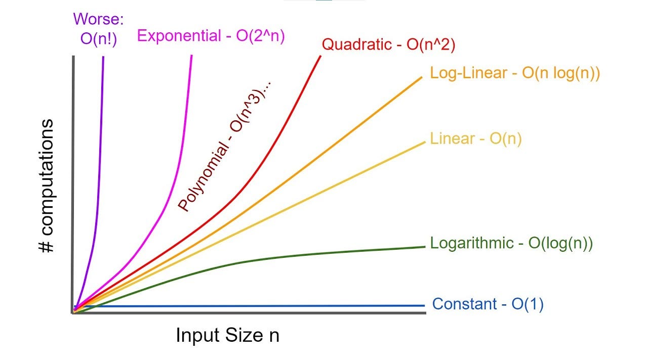
The most commonly used notation to express this kind of relationship is Big O notation, which describes an upper bound on the number of operations relative to the size of the input data. This notation represents the worst-case scenario for the growth rate of the number of operations in the algorithm, ignoring constants and lower-order terms. For example:

• O(1) means constant time - the number of operations doesn’t depend on the data size.
• O(n) means linear time - operations grow proportionally with input size.
• O(n²) means quadratic time - operations grow with the square of input size.

But why is all this important? Understanding computational complexity in the context of ABAP allows us to identify bottlenecks in the code - places that significantly slow down program execution, such as non-optimal nested loops leading to complexity on the order of O(n²). The graph below shows a comparison of different classes of computational complexity depending on the input data size n.

How to understand time complexity in ABAP - and what is the "performance killer"?

You don’t need to fully grasp the formal definition of time complexity to feel the difference between processing 10 records and 10,000... inside a nested loop. Here’s a classic “performance killer” example in ABAP:

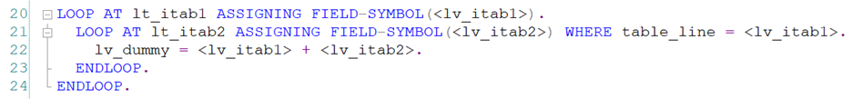
In the code above, lt_itab1 and lt_itab2 are two internal tables (lists of integers from 1 to 10,000):

The algorithm searches for common elements between the two lists in a very naive way. For each element in the internal table lt_itab1, the entire table lt_itab2 is searched (even using a WHERE clause still results in a linear search, so it doesn’t improve the algorithm's performance). For tables of equal size, the cost of such a procedure is O(n²), where n is the number of elements in each table. This code becomes inefficient for large datasets, making it difficult to scale the application - as the data grows, the execution time increases dramatically (quadratically). The runtime of this algorithm, measured using the GET RUN TIME statement, is 35,286 ms in this case.

In the following sections, we’ll show how to implement the same functionality much more efficiently using sorted tables and hashed tables.

How to improve ABAP code performance

The nested loop problem shown above can be easily solved by using sorted tables and hashed tables.

1. Sorted Tables

The following code performs exactly the same task as the first example, but uses a sorted table lt_itab2:

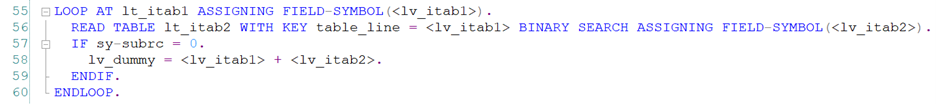
A sorted table is a special type of internal table in which the data is automatically maintained in ascending order, according to a specified sort key. In our case, the table contains a single column of integer type (recall that the data in our example consists of natural numbers ranging from 1 to 10,000), so the natural choice for the key is table_line, i.e., the value of the number itself. Thanks to this ordering, it is possible to perform fast lookups using the binary search algorithm. Binary search is an algorithm used to locate an element in a sorted array. It is based on the divide-and-conquer method and operates in O(log n) time, where n is the number of elements in the table.

And since we are searching through lt_itab2 for each of the n elements of lt_itab1, the total time complexity of the operation is O(n log n) - which is a significant improvement compared to the O(n²) complexity of the nested loop version. Indeed, when comparing execution times, this version of the algorithm completes in 5,903 ms, which is almost 6 times faster than the naive implementation.

2. Hashed tables

The fastest way to implement the functionality shown in the previous examples is by using a hashed table, as demonstrated in the example below:

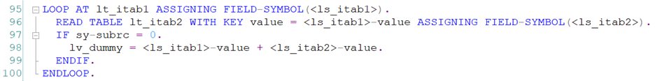
In this case, lt_itab1 is a standard internal table, whereas lt_itab2 is a hashed table.

For hashed tables, you need to explicitly define the structure of the record with a key, because you cannot use the technical alias table_line, as was possible in sorted tables. A hashed table works based on a hash function. The key value (e.g., an integer value) is transformed into a so-called hash address, which indicates exactly where the record is stored in memory. Thanks to this, the cost of accessing such an element occurs in constant time, i.e., O(1).

In our example, for every element of the table lt_itab1, a corresponding element from the table lt_itab2 is read exactly once - therefore, the time complexity of the entire algorithm in this case is linear O(n), which is the fastest among all presented. Indeed, the execution time of the algorithm in this case was 4,309 ms, showing a significant improvement compared to previous implementations.

Summary

By consciously choosing data structures such as sorted tables or hash tables, we can significantly speed up the performance of applications and avoid typical “performance killers,” such as nested loops with quadratic time complexity. In the SAP world, where business data can number in the millions of records, even a small change from O(n²) to O(n log n) or from O(n log n) to O(n) has a measurable impact on users’ working time.

‍